
XGBoost Hyperparameter tuning: XGBRegressor (XGBoost Regression)
Published:
XGBoost stands for Extreme Gradient Boosting, is a scalable, distributed gradient-boosted decision tree (GBDT) machine learning library. It provides parallel tree boosting and is the leading machine learning library for regression, classification, and ranking problems (“Nvidia”).
In this tutorial, we will discuss regression using XGBoost. We will develop end to end pipeline using scikit-learn Pipelines()and ColumnTransformer(). We will also tune hyperparameters for XGBRegressor() inside the pipeline.
Additionally, we will also discuss Feature engineering on the NASA airfoil soil noise dataset from the UCI ML repository. You can download the data using the following link.
DataLink: https://archive.ics.uci.edu/ml/machine-learning-databases/00291/airfoil_self_noise.dat
Donor:
Dr Roberto Lopez
robertolopez ‘@’ intelnics.com
Intelnics
Creators:
Thomas F. Brooks, D. Stuart Pope and Michael A. Marcolini NASA
Data Set Information:
The NASA data set comprises different size NACA 0012 airfoils at various wind tunnel speeds and angles of attack. The span of the airfoil and the observer position were the same in all of the experiments.
Attribute Information:
This problem has the following inputs:
- Frequency, in Hertzs.
- Angle of attack, in degrees.
- Chord length, in meters.
- Free-stream velocity, in meters per second.
- Suction side displacement thickness, in meters.
The only output is:
- Scaled sound pressure level, in decibels.
What you will learn?
Different EDA techniques: Histogram, Q-Q plot, Heatmap and correlation plot, Box-plot
Data Preprocessing and Feature Transformation : box-cox transformation, QuantileTransformer, KBinsDiscretizer etc.
Scikit-learn pipelines with ColumnTransformers
XGBoost Regression with Scikit-learn pipelines with ColumnTransformers
Hyper parameter tuning for XGBoostRegressor() using scikit-learn pipelines
Different regression metrics: r2_score, MAE, MSE.
Bonus: sweetviz library
How to tune XGBRegressor() using RandomizedSearchCV()
- Download data and Install xgboost.
!wget https://archive.ics.uci.edu/ml/machine-learning-databases/00291/airfoil_self_noise.dat
!pip install xgboost
--2022-03-09 15:04:32--  https://archive.ics.uci.edu/ml/machine-learning-databases/00291/airfoil_self_noise.dat
Resolving archive.ics.uci.edu (archive.ics.uci.edu)... 128.195.10.252
Connecting to archive.ics.uci.edu (archive.ics.uci.edu)|128.195.10.252|:443... connected.
HTTP request sent, awaiting response... 200 OK
Length: 59984 (59K) [application/x-httpd-php]
Saving to: ‘airfoil_self_noise.dat’

airfoil_self_noise. 100%[===================>]  58.58K  --.-KB/s    in 0.1s

2022-03-09 15:04:33 (417 KB/s) - ‘airfoil_self_noise.dat’ saved [59984/59984]

Requirement already satisfied: xgboost in /usr/local/lib/python3.7/dist-packages (0.90)
Requirement already satisfied: scipy in /usr/local/lib/python3.7/dist-packages (from xgboost) (1.4.1)
Requirement already satisfied: numpy in /usr/local/lib/python3.7/dist-packages (from xgboost) (1.21.5)
- Read the downloaded data in the pandas dataframe.
import pandas as pd
df = pd.read_table("airfoil_self_noise.dat", header = None)
df.columns =['freq', 'angle','chord','velocity','thickness','soundpressure']
df.head()
| freq | angle | chord | velocity | thickness | soundpressure | |
|---|---|---|---|---|---|---|
| 0 | 800 | 0.0 | 0.3048 | 71.3 | 0.002663 | 126.201 |
| 1 | 1000 | 0.0 | 0.3048 | 71.3 | 0.002663 | 125.201 |
| 2 | 1250 | 0.0 | 0.3048 | 71.3 | 0.002663 | 125.951 |
| 3 | 1600 | 0.0 | 0.3048 | 71.3 | 0.002663 | 127.591 |
| 4 | 2000 | 0.0 | 0.3048 | 71.3 | 0.002663 | 127.461 |
- To prevent leakage in train and test data let’s first split data into train and test set using the scikit-learn
train_test_split.
from sklearn.model_selection import train_test_split
X_train, X_test, y_train, y_test = train_test_split( df.drop(['soundpressure'], axis = 1) , df['soundpressure'], test_size=0.2, random_state=0)
Exploratory data analysis (EDA) on airfoil data.
- Since it is a regression problem, let’s plot the histogram and QQ-plot to visualize data distribution.
Linear models assume that the independent variables are normally distributed. If this assumption is not met algorithms produce poor results.
We can determine whether a variable is normally distributed with:
- Histograms and
- Q-Q plots
A histogram is a graphical representation of the distribution of data. Whereas, In a Q-Q plot, the quantiles of the independent variable are plotted against the expected quantiles of the normal distribution. If the variable is normally distributed, the dots in the Q-Q plot should fall along a 45 degree diagonal.
import scipy.stats as stats
import matplotlib.pyplot as plt
def diagnostic_plots(df, variable):
    print("\n\n Feature name is : {}\n".format(variable))
    plt.figure(figsize=(15,6))
    plt.subplot(1, 2, 1)
    plt.title("Histogram")
    df[variable].hist(bins='auto')
    plt.subplot(1, 2, 2)
    stats.probplot(df[variable], dist="norm", plot=plt)
    plt.show()
for col in X_train.columns:
    diagnostic_plots(X_train, col)
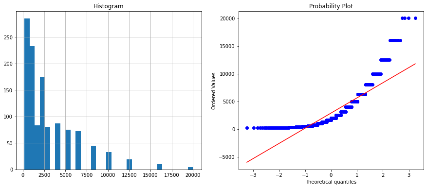
Feature name is : freq
Feature name is : angle
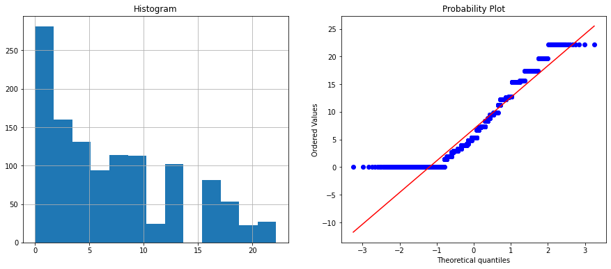
Feature name is : chord
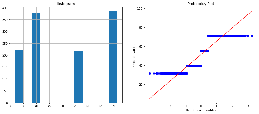
Feature name is : velocity
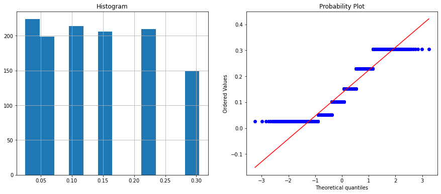
Feature name is : thickness
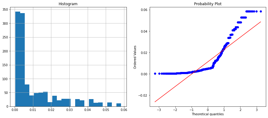
The above histogram plot shows velocity and chord features are categorical. Let’s check the unique values on these columns.
X_train.velocity.nunique(), X_test.velocity.nunique()
(4, 4)
X_train.velocity.unique()
array([71.3, 55.5, 39.6, 31.7])
X_train.chord.nunique(), X_test.chord.nunique()
(6, 6)
X_train.chord.unique()
array([0.0254, 0.2286, 0.1524, 0.1016, 0.3048, 0.0508])
The velocity column has two unique values whereas the chord column has six unique values. You can visualize it on the histogram and in the Q-Q plot.
We can directly apply label encoding on these features; because they represent ordinal data, or we can directly use both the features in tree-based methods because they don’t usually need feature scaling or transformation. However, I would like to introduce another method to encode these data called KBinsDiscretizer().
Why KBinsDiscretizer()?
Velocity and chord might change over time, and KBinsDiscretizer() can discretize the data based on clustering and encode them in an ordinal fashion. In this transformation, we will use kmeans strategy to cluster data and assign nominal values. This approach is applied if data is clustered around some number of centroids. We will take four centroids for velocity and six centroids for the chord feature.
What about other features?
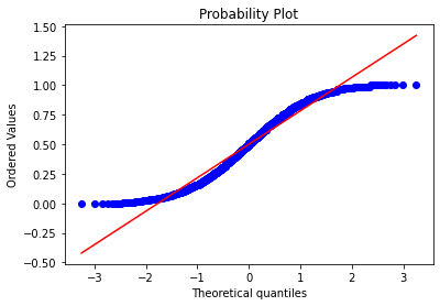
The freq feature is not normally distributed because the histogram is skewed, and the Q-Q plot does not fall along 45 degrees diagonal. Therefore we need to transform this numerical feature. There is a lot of feature transformation technique. Some of them are:
- Transforming variables with the logarithm
- Transforming variables with the reciprocal function
- Using square and cube root to transform variables
- Using power transformations on numerical variables
- Box-Cox transformation on numerical variables
- Yeo-Johnson transformation on numerical variables
A simple generalization of both the square root transform and the log transform is known as the Box-Cox transform. We will use this approach first and see the result. If the result is ok we will move on if not we will try another approach.
import seaborn as sns
train_freq , freq_lambda = stats.boxcox(X_train['freq'])
sns.distplot(train_freq)
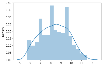
Wow! the data is now normally distributed.
Now let’s visualize the the correlation between the features on the heatmap plot.
plt.figure(figsize=(8,5))
sns.heatmap(X_train.corr(), annot = True)
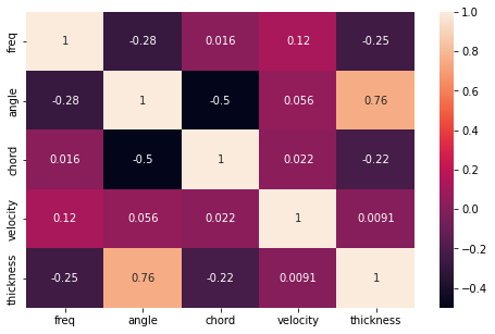
The angle and thickness features are highly correlated with score = 0.75 therefore we will drop the angle column.
X_train.drop(['angle'], axis = 1, inplace =True)
X_test.drop(['angle'], axis = 1, inplace = True)
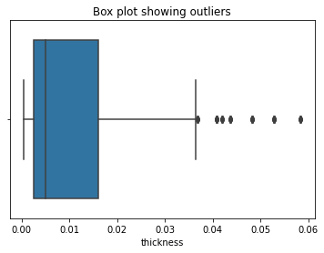
The thickness column is also highly skewed and contains outliers. Therefore we will apply QuantileTransformer() to this feature. You can learn more about QuantileTransformer() on scikit-learn.
QuantileTransformer()
- This method transforms the features to follow a uniform or a normal distribution. Therefore, for a given feature, this transformation tends to spread out the most frequent values. It also reduces the impact of (marginal) outliers: this is therefore a robust preprocessing scheme.
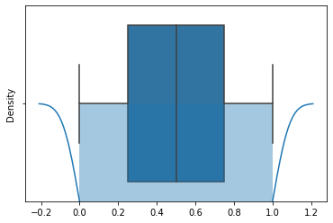
sns.boxplot(x = X_train['thickness'])
plt.title("Box plot showing outliers")
plt.show()
from sklearn.preprocessing import QuantileTransformer
scaler = QuantileTransformer()
scaler.fit(X_train[['thickness']])
train_thickness = scaler.transform(X_train[['thickness']]).flatten()
sns.distplot(train_thickness)
sns.boxplot(x = train_thickness)
stats.probplot(train_thickness, dist="norm", plot=plt)
The data is about normally distributed. The outliers has been handled.
Feature Engineering and Transformation on airfoil data based on EDA
The training data contains [freq, chord, velocity, thickness] features. From EDA we have to apply following transformations in each features.
freq: Box-cox Transformationchord: KBinsDiscretizer with 6 binsvelocity: KBinsDiscretizer with 4 binsthicknessQuantileTransformer
To apply individual transformation on features we need scikit-learn ColumnTransformer().
- Let’s first Import all necessary library
from sklearn.compose import ColumnTransformer
from sklearn.preprocessing import PowerTransformer
from sklearn.preprocessing import QuantileTransformer
from sklearn.preprocessing import KBinsDiscretizer
from sklearn.metrics import r2_score, mean_squared_error, mean_absolute_error, mean_absolute_error
import xgboost as xgb
X_train.head(2)
| freq | chord | velocity | thickness | |
|---|---|---|---|---|
| 1058 | 800 | 0.0254 | 71.3 | 0.004207 |
| 408 | 315 | 0.2286 | 55.5 | 0.011171 |
- Apply ColumnTransformer in each column. Remember, we have to specify column index to let the transformer know which transformation to apply on what column.
Here [0] means freq, [1] means chord … and so on.
transformer = ColumnTransformer(transformers=[
    ('freq',PowerTransformer(method='box-cox', standardize=False),[0]),
    ('chord', KBinsDiscretizer(n_bins = 6, encode='ordinal', strategy='kmeans'),[1] )
    ('vel',KBinsDiscretizer(n_bins = 4, encode='ordinal', strategy='kmeans'),[2]),
    ('thickness',QuantileTransformer(),[3]),
    ],
    remainder='passthrough'
    )
- Now, we have to apply XGBoost Regression on our data. Hence, we need to integrate
XGBRegressor()andColumnTransformer()object in the pipeline as shown below:
from sklearn.pipeline import Pipeline
pipe = Pipeline(steps=[("preprocessor", transformer),
                       ("model", xgb.XGBRegressor(objective= 'reg:squarederror',
                                                  learning_rate = 0.1,
                                                  n_estimators =400,
                                                  max_depth = 3,
                                                  seed = 0))])
The above approach might not give the best results because the hyperparameter is hard-coded. Therefore, need to tune hyperparameters like learning_rate, n_estimators, max_depth, etc. The two easy ways to tune hyperparameters are GridSearchCV and RandomizedSearchCV. Since RandomizedSearchCV() is quick and efficient we will use this approach here.
- We will enclose
Pipelines()insideRandomizedSearchCV()and pass necessary hyperparameters and cross validate the results. Here we will trackr2_score.
from sklearn.model_selection import RandomizedSearchCV
hyperparameter_grid = {
    'model__n_estimators': [100, 400, 800],
    'model__max_depth': [3, 6, 9],
    'model__learning_rate': [0.05, 0.1, 0.20],
    }

pipeline = RandomizedSearchCV(
    Pipeline(steps=[("preprocessor", transformer),
                    ("model", xgb.XGBRegressor(objective= 'reg:squarederror',seed = 0))
                    ]),
    param_distributions=hyperparameter_grid,
    n_iter=20,
    scoring='r2',
    n_jobs=-1,
    cv=7,
    verbose=3)
model__ is given before each hyperparameter because the name of XGBRegressor() is model.
- let’s fit the entire pipeline on Train set.
pipeline.fit(X_train, y_train)
Fitting 7 folds for each of 20 candidates, totalling 140 fits
What are the best hyperparameters?
hyperparam = pipeline.best_params_
print("The best Hyperparameters for XGBRegressor are: {}".format(hyperparam))
The best Hyperparameters for XGBRegressor are: {'model__n_estimators': 800, 'model__max_depth': 9, 'model__learning_rate': 0.05}
what is the accuracy of the model?
print("Accuracy = {} ".format(pipeline.score(X_test, y_test)))
Accuracy = 0.9586400481884366
Other Regression metrics
ypred = pipeline.predict(X_test)
print("r2_score : ", r2_score(ypred, y_test.values))
print("MSE: ", mean_squared_error(ypred, y_test.values))
print("MAE: ", mean_absolute_error(ypred, y_test.values))
r2_score :  0.9544870993856739
MSE:  1.9455311810660134
MAE:  0.9118466592072646
Bonus
!pip install sweetviz
Collecting sweetviz
Downloading sweetviz-2.1.3-py3-none-any.whl (15.1 MB)
[K |████████████████████████████████| 15.1 MB 13.8 MB/s
Installing collected packages: sweetviz
Successfully installed sweetviz-2.1.3
We can compare distribution of data on train set and test set using sweetviz.
import sweetviz as sv
report = sv.compare([X_train, "train data"], [X_test, "test data"])
report.show_html()
report.show_notebook(w="100%", h="full") # if working in colab
Report SWEETVIZ_REPORT.html was generated! NOTEBOOK/COLAB USERS: the web browser MAY not pop up, regardless, the report IS saved in your notebook/colab files.
Click this link to see the output: Link SweetViz Output
References
Galli, S. (2020). Python feature engineering cookbook: over 70 recipes for creating, engineering, and transforming features to build machine learning models. Packt Publishing Ltd.
Zheng, A., & Casari, A. (2018). Feature engineering for machine learning: principles and techniques for data scientists. “ O’Reilly Media, Inc.”.
https://scikit-learn.org/stable/modules/classes.html#module-sklearn.preprocessing
https://scikit-learn.org/stable/auto_examples/compose/plot_column_transformer_mixed_types.html#sphx-glr-auto-examples-compose-plot-column-transformer-mixed-types-py